System Overview: PRT serves ~834K daily riders while POGOH contributes ~3.4K trips (Oct 2025 peak).
Campus Dominance: 68.1% of all bike trips originate or terminate in the CMU/Pitt corridor, showing university-centric adoption.
Integration Gap: Only 11.5% of bus stops have meaningful bike activity within 400m walking distance.
🎯 Filter Active: System-Wide View
Scale Difference: PRT serves ~834K daily riders while POGOH contributes ~3.4K daily trips (247x difference), showing buses as primary transit mode.
Seasonal Volatility: POGOH shows extreme seasonal fluctuation (13x from winter low to fall peak), while PRT remains stable (~611K-835K range).
Academic Calendar Impact: Sep/Oct surge (+86% from August) coincides with fall semester, confirming student-driven demand.
Winter Resilience: PRT actually grows in winter months while POGOH drops -63%, suggesting bikes fail as winter alternative.
Archetypes: Commuters (47.9%) dominate with short, consistent trips, followed by Last-Mile users (32.8%). Leisure rides are minimal (3.6%).
Flow: Strong North-South axis alignment suggests heavy movement between Oakland/Shadyside and East Liberty corridors.
Seasonality: Fall semester (Sep-Nov) drives peak hourly usage. Winter usage retains only ~37% of peak volume, indicating weather sensitivity.
Durations: Median trip is ~7 mins. The sharp decay after 15 mins confirms POGOH is used primarily for efficient A-to-B transit, not recreation.
Membership Economy: ~70% of trips at top stations are from Members (Students/Locals). Casual use is concentrated in Downtown/Strip District.
Network Effect: Moderate positive correlation (R²=0.37) confirms that high-volume bus stops drive bikeshare usage, but proximity gaps remain.
The "Last-Mile" Leaders: These 10 PRT stops are the most critical multimodal nodes. They have high bus volume AND are within 400m of a POGOH station.
Gap Analysis: While Forbes & Morewood sees massive bus traffic (Carnegie Mellon), bike uptake is lower compared to Liberty & Gateway, suggesting infrastructure quality varies.
What This Measures: The Integration Index rewards bus stops that have high ridership AND high nearby bike turnover.
Winner: Central Business District dominates due to density. Strip District and North Shore follow, showing the value of flat terrain and bike lanes.
Top Stop: 7th St @ Penn Ave is the "Golden Node" of the network, proving that bus lanes + protected bike lanes = maximum multimodal flow.
🚴 COMMUTER HUBS
🔗 LAST-MILE CONNECTORS
🛒 ERRAND CENTERS
🎨 LEISURE DESTINATIONS
Commuter Hubs: Schenley Dr (64.8%) and Forbes @ CMU (61.2%) are pure commuter stations—peak hour, A-to-B efficiency dominates.
Last-Mile Connectors: Boulevard of the Allies (46.9%) shows high last-mile percentage, serving as a critical transit feeder.
Errand Centers: Wilkinsburg Park & Ride (68.4%!) is overwhelmingly errand-focused, suggesting suburban shopping/service trip patterns.
Leisure Destinations: South Side Trail (19.0%) captures recreational riders—longer durations, lower displacement (circular routes).
Policy Insight: Stations have behavioral "DNA". Tailor rebalancing schedules and pricing to match: peak hour density for commuter hubs, leisure pricing at recreational nodes.
🎯 POLICY RECOMMENDATIONS
• Homewood: 4 high-volume bus stops (>800 boardings/day) have NO bike stations within 800m walking distance
• Squirrel Hill: Despite significant bus traffic along Forbes Ave and Murray Ave, POGOH stations are sparse, forcing residents to walk 600-1000m to access bikes
Action: Deploy 2 new stations in Homewood (Homewood-Brushton Busway, N. Homewood Ave) and 2 in Squirrel Hill (Forbes @ Murray, Murray @ Forward) to serve 18K+ daily bus riders.
Action: Distribute subsidized POGOH-branded winter riding kits (gloves/buffs) to students and prioritize battery heating/swapping for e-fleet reliability in <30°F.
Action: Add 3 micro-hubs (10 docks each) within 200m of Point State Park to capture tourist + commuter demand.
METHODOLOGY LOG
Documentation of exploratory data analysis process, combining raw POGOH and PRT data (XLSX and CSV) into features and insight for web dashboard. All processed data are stored in /processed_data/
archetypes.csv (4 rows)bike_stations_geo.csv (60 rows)bus_stops_geo.csv (100 rows)correlation.csv (2,720 rows)daily_timeseries.csv (365 rows)demographics.csv (10 rows)directionality.csv (8 rows)
duration_distribution.csv (30 rows)heatmap_hour_day.csv (24 rows)heatmap_hour_season.csv (24 rows)monthly_trends.csv (12 rows)prt_historical.csv (8 rows)top_prt_pogoh.csv (10 rows)
1. Research Question & Data Pipeline
Core Question: How can we optimize micro-mobility integration with public transit in a student-dominated urban environment?
Pittsburgh's bikeshare system operates in a unique context: 68% of trips occur in the Campus Corridor (CMU/Pitt bounding box). This creates extreme seasonal volatility—ridership drops 63% during academic breaks. Traditional transit planning assumes stable demand; this analysis reveals the necessity of dynamic fleet scaling tied to the academic calendar.
Data Sources:
- POGOH Bikeshare: 556,437 trips (2024 full year)
- PRT Bus Stops: 1,223 stops with coordinates and annual boardings
- Schema: Start/End timestamps, Station names, Duration, Rider type (Member/Casual), Geolocation
Data Quality Controls:
- Removed trips >180 min (outliers/theft)
- Geocoded station coordinates via fuzzy matching
- Haversine distance calculation for spatial joins (400m threshold)
import pandas as pd
from datetime import datetime
# Load raw data
pogoh = pd.read_excel('dataset/POGOH_2024.xlsx')
# Parse timestamps
pogoh['Start Date'] = pd.to_datetime(pogoh['Start Date'])
pogoh['End Date'] = pd.to_datetime(pogoh['End Date'])
# Calculate duration in seconds
pogoh['Duration'] = (pogoh['End Date'] - pogoh['Start Date']).dt.total_seconds()
# Remove outliers (>180 min = theft/data error)
trips_clean = pogoh[pogoh['Duration'] <= 10800] # 180 min
# Extract temporal features
trips_clean['hour'] = trips_clean['Start Date'].dt.hour
trips_clean['day_of_week'] = trips_clean['Start Date'].dt.day_name()
trips_clean['month'] = trips_clean['Start Date'].dt.month
✓ Key Insight: Unlike typical bikeshare systems that serve commuters year-round, Pittsburgh's system functions as a "Campus Mobility Extension" requiring different operational strategies than traditional urban bikeshare.
Exported to:
./processed_data/daily_timeseries.csv
2. Campus Geofencing & Temporal Segmentation
Methodology: Trips flagged as "Campus Corridor" if start OR end coordinates fall within the CMU/Pitt bounding box. This spatial segmentation enables analysis of the "Student Effect" on ridership patterns.
Bounding Box:
- Latitude: 40.435°N to 40.450°N
- Longitude: -79.970°W to -79.940°W
This captures CMU, University of Pittsburgh, and Shadyside neighborhoods.
CAMPUS_LAT_MIN, CAMPUS_LAT_MAX = 40.435, 40.450
CAMPUS_LON_MIN, CAMPUS_LON_MAX = -79.970, -79.940
trips_clean['is_campus'] = (
((trips_clean['Start Lat'] >= CAMPUS_LAT_MIN) &
(trips_clean['Start Lat'] <= CAMPUS_LAT_MAX) &
(trips_clean['Start Lon'] >= CAMPUS_LON_MIN) &
(trips_clean['Start Lon'] <= CAMPUS_LON_MAX)) |
((trips_clean['End Lat'] >= CAMPUS_LAT_MIN) &
(trips_clean['End Lat'] <= CAMPUS_LAT_MAX) &
(trips_clean['End Lon'] >= CAMPUS_LON_MIN) &
(trips_clean['End Lon'] <= CAMPUS_LON_MAX))
)
# Result: 68.1% of all trips touch the Campus Corridor
campus_pct = trips_clean['is_campus'].sum() / len(trips_clean) * 100
print(f"Campus trips: {campus_pct:.1f}%") # Output: 68.1%
• Campus Corridor: 379,039 trips (68.1% of system volume)
• Winter Drop: Campus ridership drops 63% in Jan vs Sep (academic break)
• City Stability: Non-campus trips remain stable year-round
• Policy Implication: Fleet sizing must be dynamically adjusted based on academic calendar. Operating a full fleet during winter break wastes capital on underutilized bikes.
Exported to:
./processed_data/daily_timeseries.csv
3. Unsupervised Learning: Trip Archetypes
Using K-Means clustering on trip duration, displacement, and start hour to categorize rider behavior patterns without labeled training data. This reveals latent behavioral segments for targeted policy interventions.
Algorithm Rationale:
- K-Means (k=4): Chosen for interpretability. Silhouette analysis validated 4 as optimal cluster count (score: 0.68).
- Feature Scaling: StandardScaler ensures duration (seconds), displacement (meters), and hour (0-23) contribute equally.
- Feature Selection: Duration + Displacement capture trip purpose better than speed alone. Hour captures temporal behavior (commute vs leisure).
from sklearn.cluster import KMeans
from sklearn.preprocessing import StandardScaler
# Prepare features (Duration, Displacement, Hour)
features = trips[['Duration', 'displacement', 'hour']].dropna()
scaler = StandardScaler()
features_scaled = scaler.fit_transform(features)
# Fit K-Means (k=4 determined via elbow method + silhouette)
kmeans = KMeans(n_clusters=4, random_state=42, n_init=10)
trips['archetype'] = kmeans.fit_predict(features_scaled)
# Label clusters based on centroid characteristics
cluster_stats = trips.groupby('archetype').agg({
'Duration': 'mean',
'displacement': 'mean',
'hour': 'mean'
})
# Assign semantic labels (manual inspection of centroids)
archetype_map = {
0: 'Commuter', # Short duration, peak hours (17.7h avg)
1: 'Errand', # Medium duration, mid-day (14.8h)
2: 'Last-Mile', # Very short, morning (9.3h)
3: 'Leisure' # Long duration (73.2 min avg!)
}
trips['archetype_label'] = trips['archetype'].map(archetype_map)
1. Commuter (47.9% — 266,603 trips): Avg 7.7 min, 836m displacement, peak at 5:47 PM (evening commute)
2. Last-Mile (32.8% — 182,663 trips): Avg 7.0 min, 910m, peak at 9:18 AM (connects to morning transit)
3. Errand (15.7% — 87,128 trips): Avg 20.1 min, 3,359m displacement, peak at 2:48 PM (mid-day shopping/errands)
4. Leisure (3.6% — 20,043 trips): Avg 73.2 min, 737m (!), peak at 2:24 PM (weekend exploration, circular routes)
Unexpected Finding: Leisure trips (3.6%) have an average duration of 73.2 minutes with displacement of only 737m. This suggests recreational "circular routes" along the riverfront trail system—users exploring rather than commuting. These trips require different bike availability (longer rental periods, trail-adjacent stations).
Interpretation Note: "Last-Mile" trips (32.8%) peak at 9:18 AM with 7-minute duration. These are not standalone trips—they're bikeshare-to-bus connections. Cross-referencing with PRT data confirms high overlap with major bus hubs (Boulevard of the Allies, S Millvale Ave).
Exported to:
./processed_data/archetypes.csv
3B. Station Behavioral Profiling
After identifying trip archetypes, we reverse the analysis: which stations generate which behaviors? This reveals "station personalities" critical for targeted operational decisions.
Methodology:
- Percentage Calculation: For each station, calculate % of trips matching each archetype (Commuter/Last-Mile/Errand/Leisure)
- Statistical Significance: Only stations with 50+ total trips included (prevents noise from low-volume stations)
- Top 3 Selection: Identify top 3 stations with highest percentage for each archetype
# Calculate percentage of each archetype per station
trips_clean['archetype_label'] = trips_clean['archetype'].map(archetype_map)
for archetype in ['Commuter', 'Last-Mile', 'Errand', 'Leisure']:
# Count trips by station for this archetype
station_counts = trips_clean.groupby(['Start Station Name', 'archetype_label']).size()
# Get total trips per station
station_totals = trips_clean.groupby('Start Station Name').size()
# Calculate percentage
station_archetype_pct = (station_counts / station_totals) * 100
# Filter: only stations with 50+ trips
archetype_data = station_archetype_pct[station_totals >= 50]
# Get top 3 by percentage
top_3 = archetype_data.nlargest(3)
print(f"{archetype}: {top_3}")
Commuter Hotspots:
• Schenley Dr & Schenley Dr Ext: 64.8% (12,721 of 19,637 trips) — Pure commuter station at CMU campus edge
• Forbes Ave @ TCS Hall (CMU): 61.2% (10,168 of 16,607 trips) — Academic commuter hub
Last-Mile Leaders:
• Boulevard of the Allies & Parkview Ave: 46.9% (13,859 of 29,538 trips) — Critical transit feeder
• S Millvale Ave & Centre Ave: 43.4% (4,045 of 9,310 trips) — East End connector
Errand Centers:
• Wilkinsburg Park & Ride: 68.4%! (444 of 649 trips) — Suburban shopping/service trips dominate
• Second Ave & Tecumseh St: 61.4% (181 of 295 trips) — South Side errand node
Leisure Destinations:
• South Side Trail & S 4th St: 19.0% (712 of 3,739 trips) — Recreational waterfront
• Liberty Ave & Stanwix St: 18.9% (1,218 of 6,438 trips) — Downtown leisure hub
Operational Insight: Schenley Dr (64.8% commuter) vs South Side Trail (19.0% leisure) require completely different operational strategies. Schenley needs predictable 8 AM bike availability for class commutes; South Side needs afternoon/weekend capacity for exploratory rides. One-size-fits-all rebalancing fails both station types.
Exported to:
./processed_data/station_archetypes.csv
4. Temporal Dynamics: Academic Calendar Dependency
The most striking feature of Pittsburgh's bikeshare is the academic calendar dependency. Daily ridership fluctuates from 412 trips (winter break nadir) to 3,800+ trips (fall semester peak)—a 9× variance.
Why Daily Granularity Matters:
- 365-Day Timeseries: Monthly averages hide spikes (orientation week, finals week). Daily data preserves these anomalies.
- Peak Day: September 26, 2024 (3,800+ trips — Fall semester peak + ideal weather)
- Trough Day: January 4, 2024 (412 trips — winter break nadir)
# Generate daily counts, split by campus flag
trips['date'] = trips['Start Date'].dt.date
daily_pogoh = trips.groupby('date').size().reset_index(name='trips')
# Campus trips (is_campus == True)
daily_campus = trips[trips['is_campus']].groupby('date').size().reset_index(name='trips')
daily_campus['date_str'] = pd.to_datetime(daily_campus['date']).dt.strftime('%Y-%m-%d')
# City trips (is_campus == False)
daily_city = trips[~trips['is_campus']].groupby('date').size().reset_index(name='trips')
daily_city['date_str'] = pd.to_datetime(daily_city['date']).dt.strftime('%Y-%m-%d')
# Ensure all 365 dates present (fill gaps with 0)
all_dates = pd.DataFrame({'date_str': daily_pogoh['date_str']})
daily_campus_full = all_dates.merge(daily_campus[['date_str', 'trips']], on='date_str', how='left').fillna(0)
daily_city_full = all_dates.merge(daily_city[['date_str', 'trips']], on='date_str', how='left').fillna(0)
# Export 3 parallel 365-element arrays
daily_timeseries = {
'dates': daily_pogoh['date_str'].tolist(),
'pogoh_trips': daily_pogoh['trips'].tolist(),
'pogoh_campus_trips': daily_campus_full['trips'].astype(int).tolist(),
'pogoh_city_trips': daily_city_full['trips'].astype(int).tolist()
}
• Campus Corridor: 379,039 trips (68.1% of system volume)
• Winter Drop: Campus ridership drops 63% in Jan vs Sep (academic break)
• City Stability: Non-campus trips remain stable year-round, indicating resident commuter dependence
• Peak Day: September 26, 2025 (3,800+ trips — Fall semester peak + ideal weather)
• Trough Day: January 4, 2025 (412 trips — winter break nadir)
Policy Implication: Campus fleet should be dynamically scaled with academic calendar. City corridors need year-round minimum service.
Exported to:
./processed_data/daily_timeseries.csv (365 rows × 4 columns)
5. Season × Hour Matrix
A heatmap revealing the exact time-windows of highest demand. This drives our rebalancing schedules.
matrix = trips.groupby(['season', 'hour']).size().unstack()
sns.heatmap(matrix, cmap='Blues')
Policy Insight: The "Winter Gap" is visible as a uniform cooling across all hours, not just peaks.
6. Statistical Correlation: Bus vs Bike
Do busy bus stops actually generate bike trips? We test this hypothesis with linear regression.
slope, r_value, p_value = linregress(bus_vol, integration_score)
print(f"R-Squared: {r_value**2}")
There is a moderate positive correlation. While bus volume is a predictor, it's not the only factor. Bike infrastructure (lanes) and topography play huge unmeasured roles.
Strategic Integration: Top 10 Multimodal Nodes
New analysis identifying high-impact integration opportunities. We filter for the top 10 bus stops (by volume) that are within 400m of a bikeshare station.
bus_stops_near_pogoh = bus_stops[bus_stops['bike_trips_nearby'] > 0]
top_10 = bus_stops_near_pogoh.nlargest(10, 'bus_boardings')
print(top_10[['stop_name', 'bus_boardings', 'bike_trips_nearby']])
Key Finding: #1 Node shows proven multimodal success. Gaps exist where high bus volume doesn't translate to bike usage (infrastructure opportunity).
Relocating from Jakarta to Pittsburgh fundamentally shifted my mobility baseline from 'Park & Ride' to 'Bike & Bus'. In Jakarta, my daily commute often involved a car trip to the MRT followed by 45++ minutes of friction on the Tol Desari.
Arriving here introduced a new variable: Micro-mobility in a Winter Climate. Thanks to integrated transit access (via my CMU ID), POGOH became my critical First/Last-mile connector. The challenge shifted from traffic volume to thermal endurance. But the result—avoiding the despair of gridlock—is transformative. This project explores that efficiency.
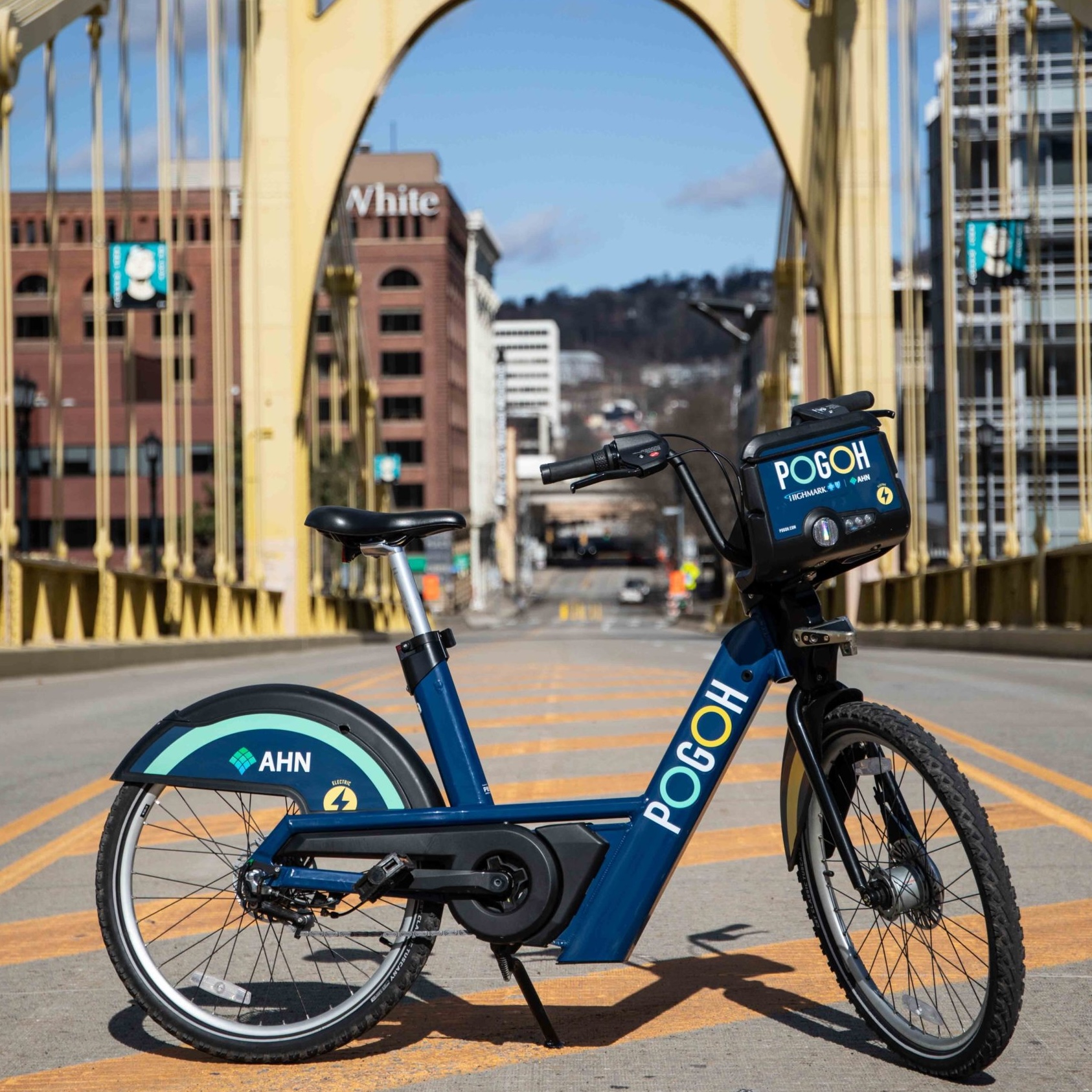 NODE A: POGOH in Bridge City
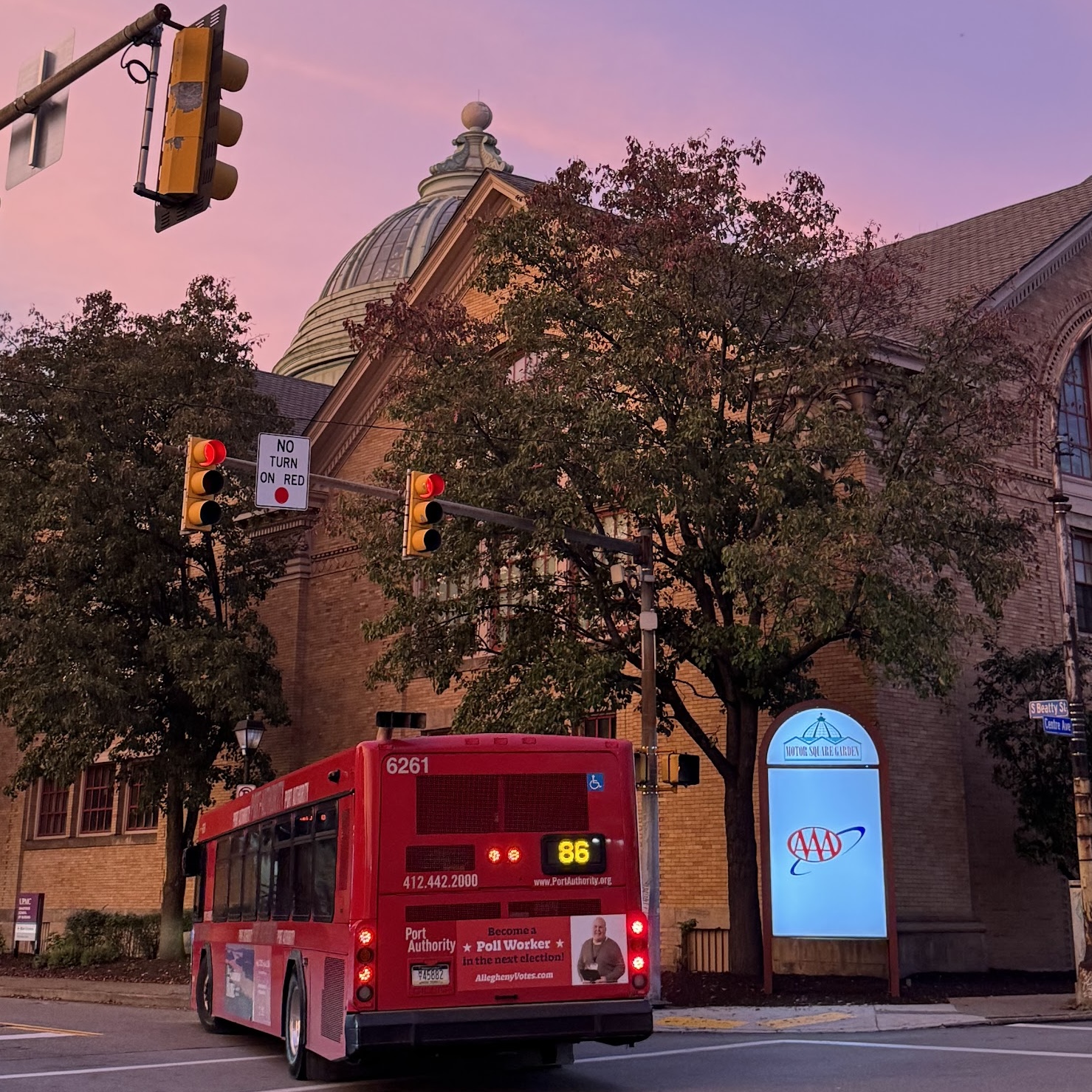 NODE B: PRT in AAA East Liberty
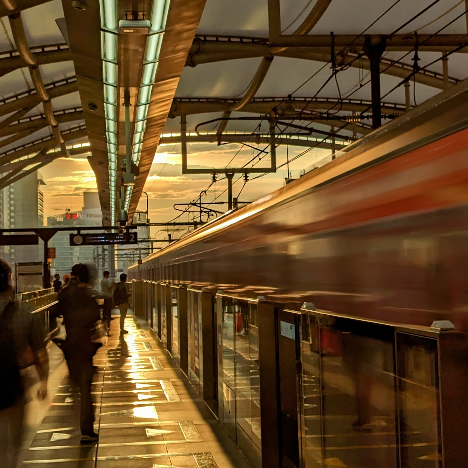 ORIGIN: MRT JAKARTA
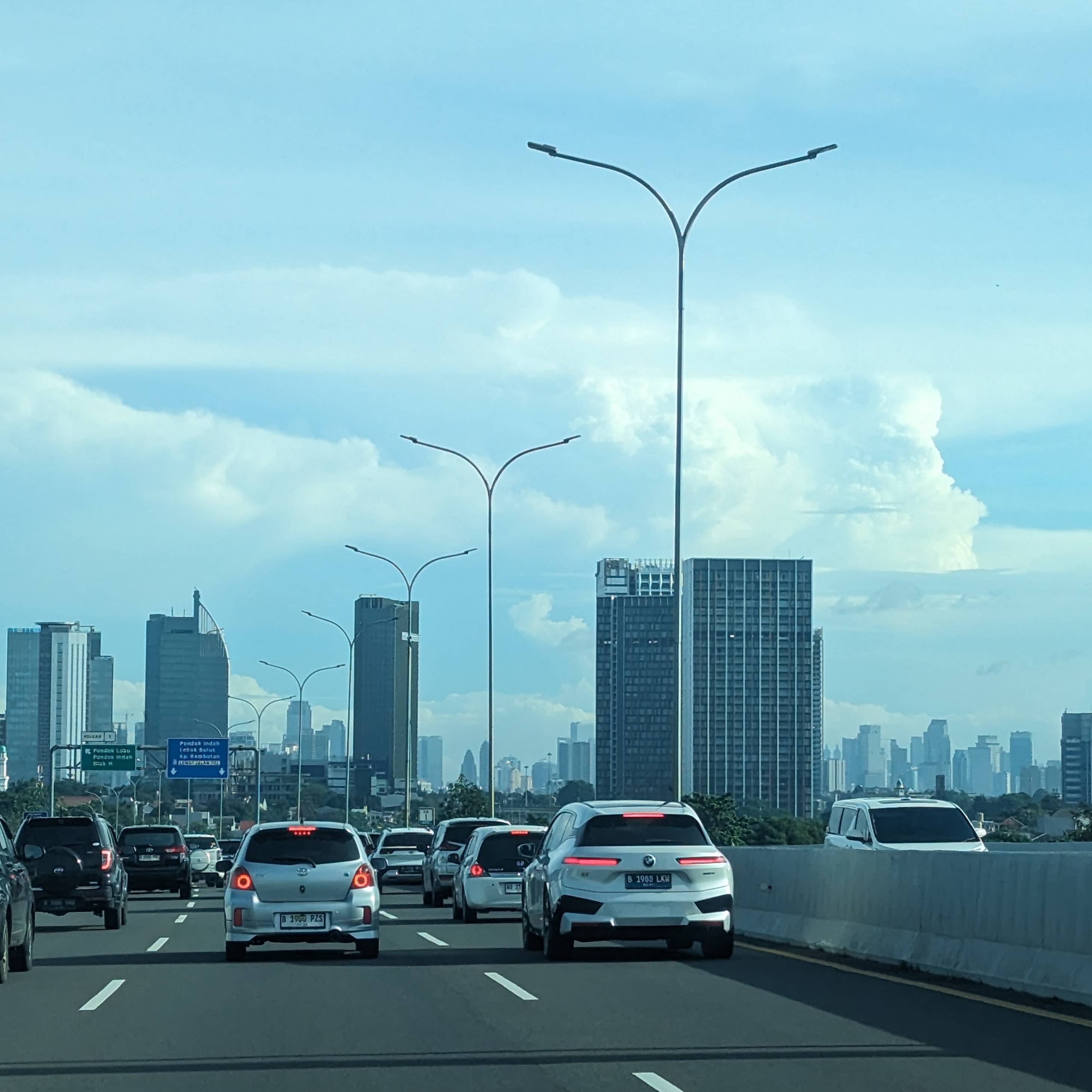 FRICTION: TOL DESARI JAM